The following graphs are generated using the 10-day scoring algorithm used by the VulnCheck vulnerability-trending index.
Top 10 Trending CVE
import os
import sys
import requests
import pandas as pd
import matplotlib.pyplot as plt
from IPython.display import HTML

# %%
# Fetch data from VulnCheck API
API_URL = "https://api.vulncheck.com/v3/index/vulnerability-trending"
VC_TOKEN = os.getenv("VULNCHECK_API_TOKEN")

if not VC_TOKEN:
    raise EnvironmentError("VULNCHECK_API_TOKEN environment variable not set")

headers = {
    "Accept": "application/json",
    "Authorization": f"Bearer {VC_TOKEN}"
}

response = requests.get(API_URL, headers=headers)
response.raise_for_status()
data = response.json()
data = data["data"]

# %%
# Extract 10-day trending CVEs
ten_day_entry = next(d for d in data if "10 Day" in d["title"])
df_10day = pd.json_normalize(ten_day_entry["cve"])

# Sort and take top 10
top10 = df_10day.sort_values(by="score", ascending=False).head(10)
top10.reset_index(drop=True, inplace=True)

# Build links to VulnCheck Console
df_display = top10.copy()
df_display["cve"] = df_display["cve"].apply(
    lambda x: f'<a href="https://console.vulncheck.com/cve/{x}" target="_blank">{x}</a>'
)

# Only keep relevant columns
df_display = df_display[["cve", "score", "inKEV", "inVCKEV"]].fillna(False)

# Render as HTML (ensures links are clickable)
HTML(df_display.to_html(escape=False, index=False))
Loading...
Evidence Breakdown
import numpy as np
import collections
import pandas as pd
import matplotlib.pyplot as plt

def tag_counts(refs):
    counter = collections.Counter()
    if not isinstance(refs, list):
        return counter
    for r in refs:
        if not isinstance(r, dict):
            continue
        for t in r.get("tags", []) or []:
            if t is None:
                continue
            counter[str(t)] += 1
    return counter

# Build per-CVE tag counts and discover the tag universe dynamically
ev_rows = []
all_tags = set()

for row in top10.to_dict(orient="records"):
    counts = tag_counts(row.get("reference_urls", []))
    all_tags |= set(counts.keys())
    counts["cve"] = row["cve"]
    ev_rows.append(counts)

if not ev_rows:
    raise ValueError("No rows to plot.")

ev = pd.DataFrame(ev_rows).fillna(0).set_index("cve")

# Ensure all discovered tags exist as columns
for t in all_tags:
    if t not in ev.columns:
        ev[t] = 0

# Convert to int (counts) and order CVEs by total evidence
ev = ev.astype(int)
ev = ev.loc[ev.sum(axis=1).sort_values(ascending=True).index]

# Optionally keep only the top K most common tags across the Top-10 set
TOP_K_TAGS = 8  # adjust or set to None to keep all
tag_totals = ev.sum(axis=0).sort_values(ascending=False)
if TOP_K_TAGS is not None and len(tag_totals) > TOP_K_TAGS:
    keep_cols = tag_totals.head(TOP_K_TAGS).index.tolist()
    ev = ev[keep_cols]
else:
    # Keep all tags, but order columns by overall frequency desc
    ev = ev[tag_totals.index.tolist()]

# If no tags made it through, bail out nicely
if ev.shape[1] == 0:
    print("No tag data available to plot.")
else:
    # Stacked horizontal bars
    plt.figure(figsize=(10, 6))
    left = np.zeros(len(ev))
    for col in ev.columns:
        plt.barh(ev.index, ev[col], left=left, label=col)
        left += ev[col].values
    plt.xlabel("Evidence Count (refs over last 10 days)")
    plt.title("Why Are These CVEs Trending?")
    plt.legend()
    plt.tight_layout()
    plt.show()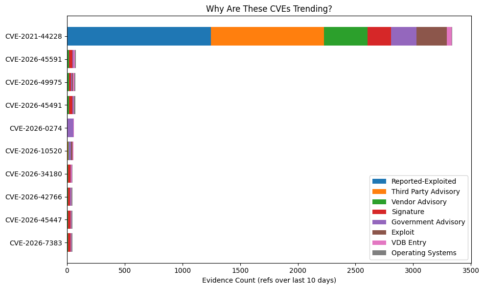
Reference Date Activity Heat Map
import datetime as dt
import numpy as np
import matplotlib.pyplot as plt
from collections import defaultdict

# Build a 10-day window ending today (or use the API’s `date_added` anchor)
end = dt.date.today()
days = [end - dt.timedelta(days=i) for i in range(9, -1, -1)]  # 10 days, oldest→newest

def hits_by_day(refs):
    s = set()
    for r in refs:
        d = r.get("date_added")
        if not d: continue
        # Parse ISO timestamp (truncate to date)
        try:
            ddate = dt.date.fromisoformat(d[:10])
        except Exception:
            continue
        s.add(ddate)
    return s

matrix = []
labels = []
for row in top10.to_dict(orient="records"):
    labels.append(row["cve"])
    s = hits_by_day(row.get("reference_urls", []))
    matrix.append([1 if d in s else 0 for d in days])

M = np.array(matrix)

plt.figure(figsize=(10,6))
plt.imshow(M, aspect="auto")
plt.yticks(range(len(labels)), labels)
plt.xticks(range(len(days)), [d.strftime("%m-%d") for d in days], rotation=45)
plt.title("10-Day Activity Heat (any reference seen on a day = 1)")
plt.xlabel("Day")
plt.ylabel("CVE")
plt.tight_layout()
plt.show()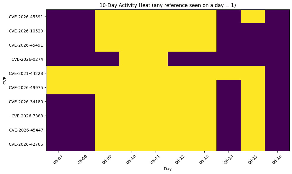
Trending Momentum
import pandas as pd
import matplotlib.pyplot as plt

# Pull both windows from your already-fetched API payload
ten = next(d for d in data if "10 Day" in d["title"])
thrty = next(d for d in data if "30 Day" in d["title"])
df10 = pd.json_normalize(ten["cve"])
df30 = pd.json_normalize(thrty["cve"])

# Rank (1 = hottest); keep only CVEs in 10-day Top-10 to reduce clutter
focus = top10["cve"].tolist()
r10 = df10.assign(rank_10=df10["score"].rank(ascending=False, method="min"))
r30 = df30.assign(rank_30=df30["score"].rank(ascending=False, method="min"))
merged = r10[["cve","rank_10"]].merge(r30[["cve","rank_30"]], on="cve", how="left")
merged = merged[merged["cve"].isin(focus)].dropna()
merged = merged.sort_values("rank_10")

# Slope plot
plt.figure(figsize=(8,6))
x0, x1 = 0, 1
for _, row in merged.iterrows():
    plt.plot([x0, x1], [row["rank_30"], row["rank_10"]], marker="o")
    plt.text(x0-0.02, row["rank_30"], row["cve"], ha="right", va="center")
plt.xticks([x0, x1], ["30-Day Rank", "10-Day Rank"])
plt.gca().invert_yaxis()  # rank 1 at top
plt.title("Momentum: 30-Day → 10-Day Rank (Top-10 Focus)")
plt.tight_layout()
plt.show()